Research, Surveys and Data Management

Nature Conservation 2026 — 20. 8. 2026 — Research, Surveys and Data Management — Print article in pdf

Ecosystem Accounting: Services by Pollinators

author: Pavel Moskaljuk

One of these services, treated in this study, is that of pollinators, i.e. the benefit of wild pollinators for the production of food crops. Even though we use controlled pollination provided by beekeepers today, wild pollinators have still been doing most of the pollination work. In the past decades, the abundance and diversity of insect pollinators (bees, butterflies, hoverflies, and moths) have declined dramatically. One of the main causes is agricultural intensification, landscape fragmentation, and other changes to the landscape, which deprive pollinators of their natural habitats and food sources (Potts et al., 2021).

For this reason, the need for a detailed statistical assessment has arisen (known as ecosystem accounting), based on the requirements of Eurostat (United Nations, version 2024-12-12), the statistical office of the European Union playing a key role in this field, particularly in the coordination of environmental data collection methods (currently in a testing phase). As of 2026, the results of this analysis will be reported every year. In this case, the best option would be in-situ monitoring, but this method is not available in the Czech Republic. Thus, insect populations need to be predicted based on assessment of the condition and extent of the ecosystems and other variables significantly influencing the lives of pollinators.

Methodological approach

The analysis is inspired by the methodological framework developed by Eurostat dealing with the identification of suitable habitats for pollinators and subsequent identification of ecosystems which contribute most to this ecosystem service. In our case, the general approach was significantly expanded to include more detailed data and more sophisticated analytical methods, enabling a highly accurate localisation of areas important for pollinators. Therefore, the main objective was to identify suitable habitats, predict areas with insufficient pollination, and forecast agricultural yields attributable to the wild pollinator activity. As the evaluation is conducted annually, the analysis was transcribed and automated using the Python programming language.

Factors/drivers affecting pollination services

• Habitat characteristics;
• Distance between food source and habitat;
• Activity of pollinating insects

To visualise the factors/drivers, the following map layers were created (described in more detail in the following chapters):

Maps of ecosystems, Significant Landscape Elements and agricultural practices;

• Maps with correction factors assessing flower attractiveness and habitats;
• Maps of air temperature and solar radiation;
• Maps eliminating unsuitable areas according to landscape fragmentation;
• Maps showing high probability of pollinator occurrence, adjusted with threshold values;
• Maps of crops dependent on pollinators;
• Maps distinguishing pollinated and non-pollinated crops;
• Maps of the most beneficial ecosystems for pollination services.

The analysis is based on spatial data from 2023 (see Tab. 1) and uses a combination of tools of the QGIS geospatial software, the Python programming language, and the Google Earth Engine Code web environment (JavaScript). All spatial calculations were performed at a grid resolution of 10 × 10 m, ensuring a high level of detail for spatial interpretation of the results.

 

Table 1. List of input datasets used, including their providers. The datasets cover various topics, ranging from geographic and environmental information to meteorological and agricultural data.

Dataset	Provider
Linear infrastructure (ZABAGED)	SALSC
Ecosystems (KVES 2023)	NCA CR
Ecologically important areas	LPIS
Land parcels	LPIS
Agricultural crops	LPIS
Air temperature	Copernicus ERAS
Solar radiation	Copernicus ERAS
Digital elevation model	SALSC

 

SALSC – State Administration of Land Surveying and Cadastre, NCA CR – Nature Conservation Agency of the Czech Republic, LPIS – Land Parcel Identification System

 

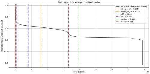
Graph 1. Finding a threshold value using several statistical methods. The model includes approx. 788,700,000 samples. Compiled by Pavel Moskaljuk.

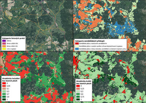
Map 1. Map display of raster data with the following variables: 1. linear element category (top left), 2. agricultural approach category (top right), 3. nesting attractiveness excl. forest areas (bottom left), 4. flower attractiveness excl. forest areas (bottom right). Southern Brdy Higlands region, vicinity of the town of Blovice (western Bohemia). Compiled by Pavel Moskaljuk.

Identifying landscape elements with positive and negative impacts on pollinators

In the first step, the analysis classified and indexed narrow linear elements in the landscape. These include particularly alleys, hedges, and baulks, as well as roads and streets. The nature of these elements is essential when identifying suitable habitats for pollinators, as it affects their movement and presence. For this reason, the layers of roads (State Administration of Land Surveying and Cadastre, SALSC) and non-agricultural linear elements was merged with the layer of ecologically significant elements (Land Parcel Identification System, LPIS). The linear elements are represented by highly detailed vectors (see Map 1). Correction factors were set as follows:

• 0 to < 1 – negative impact;
• 1 – neutral impact;
• 2 – positive impact.

Another significant factor with a major impact on pollinators is agricultural practices on cultivated land. The approach applied takes into account farming intensity and quality. For these purposes, the LPIS layer was used, which distinguishes farmland types in detail and also identifies whether organic farming is practised on a parcel. Selected areas from the ecologically significant areas (LPIS) layer were added to the layer. In the case of overlays in the raster display, the values ​​were averaged. Similar to the linear elements, agricultural practices were rated with an index from 0 to 2 (see Tab. 2), with an additional index of 0.2 for farming. The resulting data (see Map 1) can be interpreted as follows:

1. Land farmed intensively;
2. Farmland with a high rate of (semi-)natural vegetation;
3. Low-intensity farmland with small landscape elements.

Table 2. Categories of farmland linked via two input layers consisting of ecologically significant areas and parts of blocks. Correction factors serve as a basis for filling the expert model equation (described below)

Farmland category	Correction factor
Landscape orchard (Streuobstwiese)	1.3
Orchard	1.3
Permanent grassland	1.3
Thalweg grassland	1.2
Other permanent field crop	1.2
Grassland (on arable land)	1.2
Fallow land	1.2
Baulk	1
Wetland	0.75
Ditch	0.75
Group of trees and scrubs	1
Solitary tree	1
Alley	1
Terrace	1
Afforested land	0.75
Area of fast-growing trees cultivated in coppices	0.75
Other plantation	1
Nonproductive land	1
Fast-growing trees	0.75
Afforested land	0.75
Hop garden	1
Common arable land	0.75
Vineyard	1
Fishpond	0
Area with perennial production crops	0.75
Area with containers	0
Area with truffles	1
Tree nursery	1
Rock garden	0.75
if locally farmed organically + 0.2

 

 

 

For a better idea, in 2023, in the Czech Republic farmland with intensive agriculture covered an area of 24,066.3 km² (68%), while low-intensity farmland with landscape elements or natural vegetation 11,079.1 km² (31%).

In the following step, the impact of various ecosystem types on the presence and activity of pollinators was assessed. For this purpose, the Consolidated Layer of Ecosystems (CLES) layer was used (Nature Conservation Agency of the Czech Republic, NCA CR), which classifies the territory into 40 different ecosystem categories based on their ecological characteristics. Similar to the previous steps, correction factors were assigned to the ecosystems (see Tab. 3) according to two key criteria.

Table 3. Ecosystem assessment according to flower and nesting attractiveness.

Ecosystem	E1	E2
	Flower attractiveness	Nesting attractiveness
Alpine meadows	1	0.8
Alluvial and wet meadows	1	0.8
Swamp, marsh	0.55	0.1
Degraded grassland	0.5	0.7
Road network	0.25	0.3
Hop garden	0.6	1
Macrophyte vegetation of stagnant water	0	0
Urban greenery, ornamental garden, park, cemetery	0.5	0.7
Mesic meadows	1	0.8
Wetlands and riparian vegetation	0.55	0.1
Scattered built-up area	0.3	0.3
Arable land	0.4	0.05
Orchard, garden	0.9	1
Industrial and business units	0.05	0.1
Peatbogs and springs	0.5	0.1
Fishponds, lakes, reservoirs	0	0
Rocks, (artificial) quarries	0.05	0.7
Rocks, scree	0	0
Waste dumps and building sites	0	0.05
Contiguously built-up area	0.05	0.1
Sports and recreation areas	0.05	0.3
Dry grasslands	0.75	1
Vineyard	0.6	1
Streams	0	0
Heaths	1	0.7

 

 

 

kk

1. Flower attractiveness, i.e. the degree to which a particular ecosystem provides a source of food for pollinators (see Map 1).
2. Nesting attractiveness, i.e. suitability of a habitat for the nesting and shelter of pollinators (see Map 1).
3. It should be noted that forest areas have not yet been included in this step. These will be addressed in the analysis below.

 

Pollinator flight ranges

Another important input variable is the flight range of pollinators, which is a key factor in identifying suitable habitats. Simply, pollinators choose their habitats in a way that food is within easy reach. For this reason, forest ecosystems, which were excluded from assessment in the previous steps, were provided with inner mantle zones. These are used to identify forest areas which are located too far from potential food sources and are at the same time unattractive to pollinators. In this case, a flight range of 200 m was chosen, corresponding to the operation range of many wild pollinator species. In the first step, small isolated forest patches (1–2 pixels 10 × 10 m in size) were eliminated, as they could distort the analysis disproportionally. Subsequently, using Euclidean distance, the distance between each pixel representing a forest ecosystem and the nearest pixel which could represent a food source was calculated. After several adjustments and based on the previous calculation, an inner mantle zone was created, enabling the distinction of forest areas located in the immediate vicinity of suitable habitats from isolated ones and those less accessible for pollinators (Map 2).

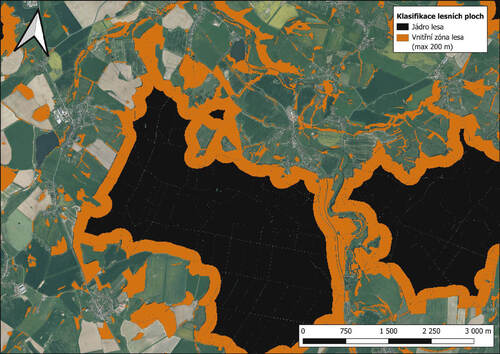
Map 2. Classification of forest areas according to 200 m flight range. Southern Brdy Highlands region, vicinity of the town of Blovice (western Bohemia). Compiled by Pavel Moskaljuk.

Map 3. Cover picture, description at the end of the article.

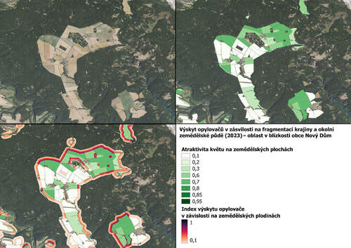
Map 4. Illustration of the impact of landscape fragmentation and flower attractiveness on agricultural land. Map sections show an area near the village of Nový Dům (Central Bohemia). Compiled by Pavel Moskaljuk.

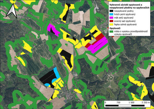
Map 5. Identifying pollinated and non-pollinated crops dependent on pollination. For identification of these areas, a 200 m flight range around sites with a high probability of pollinator occurrence was used. Compiled by Pavel Moskaljuk.

After completing the spatial classification, the forest areas were assessed according to the criteria shown in Tab. 4. Finally, they were merged with the resulting layers from the previous step.

Table 4. Correction factors for different types of forest ecosystems classified according to pollinator flight range. The table further shows the proportional distribution of categories relative to the total area of each forest ecosystem type.

Forest category	Position	Nesting attractiveness	Flower attractiveness	km²
Broad-leaved	200-m edge	1	1	4,268.8
	core	0.3	0.2	2,927.4
Coniferous	200-m edge	1	1	8,000
	core	0.2	0.2	7,259.5
Mixed	200-m edge	1	1	3,737
	core	0.3	0.2	1,517

 

 

Connection of variables to pollinator activity

Based on a detailed description of several key variables, which significantly influence the potential occurrence of pollinators, an expert index was created combining all previous indices. For this calculation, the following equation was derived using raster calculations:

where:

ek = pixel representing an ecosystem

AK = flower attractiveness 0–1

AH = nesting attractiveness 0–1

KL_ek = correction factor for linear elements

KZ_ek = correction factor for agricultural elements

KE_vp = correction factor for ecologically significant areas

EI_ek = pollinator expert index

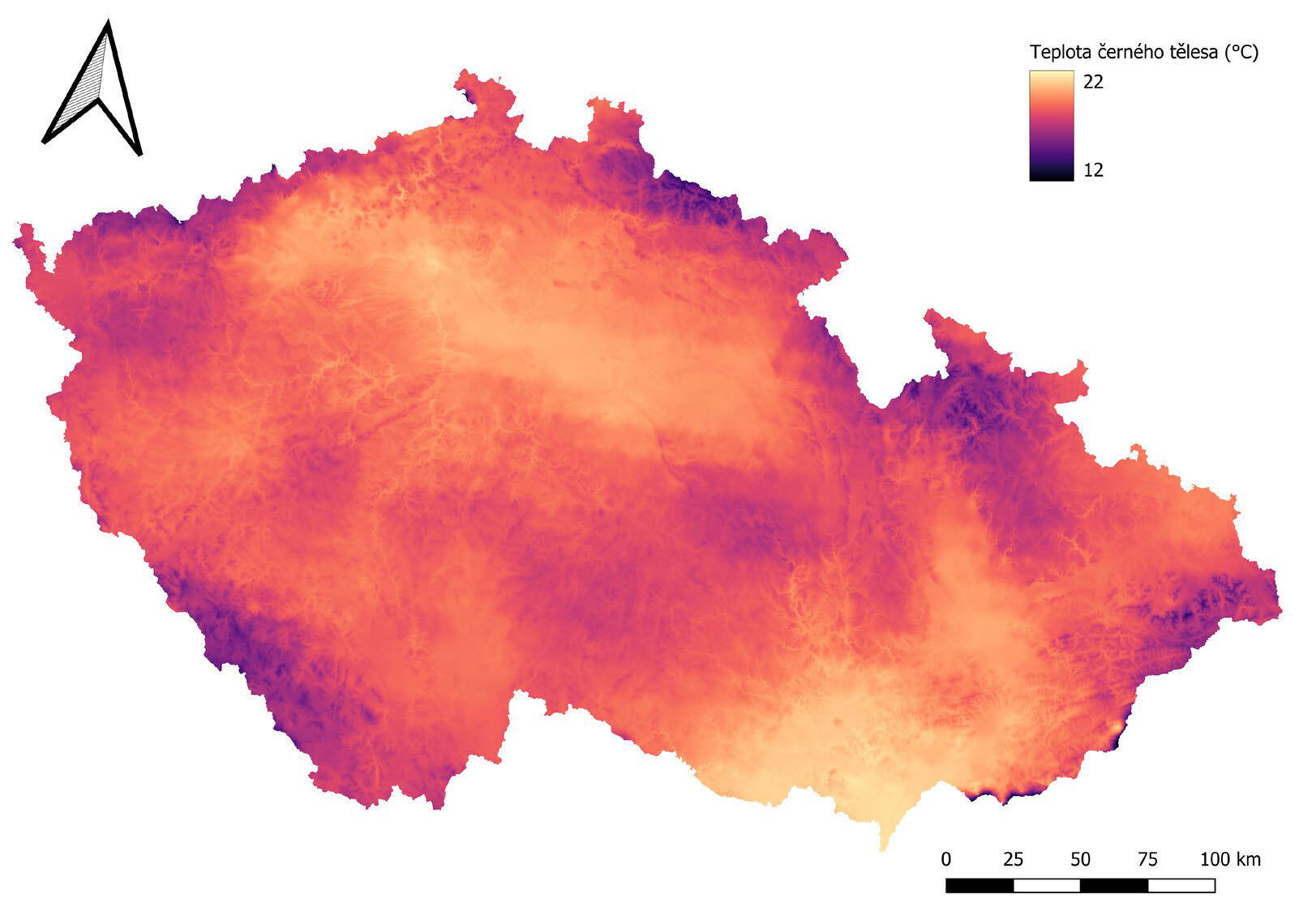
The occurrence and behaviour of insects are significantly influenced by temperature and solar radiation intensity. Insect activity generally correlates positively with these factors, with each pollinator species becoming active only when the so-called blackbody temperature (i.e. the radiant temperature perceived by the insect’s body) exceeds a certain threshold (Corbet et al. 1993). The approach allows us to simulate the temperature conditions under which insects are capable of active movement at a specific time and location.

For the calculation of blackbody temperature, two input layers from the ECMWF/ERA5_LAND/HOURLY dataset provided by the Copernicus service were used.

1. Air temperature at 2 m above the ground (1,000 × 1,000 m)
2. Short-wave solar radiation (1,000 × 1,000 m)

The data were averaged for the period April to September 2023 and only during daytime hours from 6 am to 8 pm, when we expect insect activity to be the highest. Data from cloudy days were also included.

Calculation of the blackbody temperature is based on coefficients from a British study (Corbet et al. 1993). Given the large volume of data, the calculation was performed for each day within the time interval, and finally the average for the entire observation period was calculated.

where:

T = average temperature from April to September 2023

R = average radiation from April to September 2023 (6:00–20:00)

Tčt = blackbody temperature

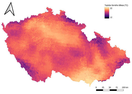
Since the input data are available only at a resolution of 1,000 × 1,000 m, one of the spatial downsampling regression methods was used to improve the accuracy. Specifically, the Kriging regression method was chosen, combining a linear regression model with spatial interpolation. Elevation data from the digital elevation model (SALSC) was used as a predictor, as elevation significantly influences temperature conditions. The result was a prediction of Tčt values at a finer resolution of 100 × 100 m, which better captures local topographic conditions (see Map 3).

Based on the calculated Tčt, the insect activity index (IA_ek) was then derived using the following equation:

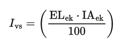
For a comprehensive assessment of the habitat suitability for pollinators, the final indicator combined the pollinator expert index (EL_ek) with the insect activity index (IAek), which provides a more accurate view of the real occurrence of pollinators based on a combination of biotic and abiotic factors:

Impact of landscape fragmentation and search for a threshold value

The result from the previous step (habitat suitability index) already provides a fairly comprehensive description of the sites/areas where pollinators are highly likely to occur. However, this leaves the issue of landscape fragmentation and the determination of a threshold value which clearly distinguishes areas with and without pollinators.

Landscape fragmentation is a key factor affecting the lives of pollinators. To assess its impact, it is first necessary to identify areas which are too far from food sources, while also taking into account the attractiveness of those sources. The basic analysis already takes into account food sources in meadows and other natural ecosystems, but a significant role is also played by agricultural crops, particularly those which are rotated in seeding practices. Therefore, all crops in the 2023 crop layer (LPIS) were assessed using attractiveness coefficients reflecting the quality and quantity of food available to pollinators. A total of 327 crops were assessed, with each assigned a coefficient based on the following rule: the larger the food supply, the higher the coefficient. For example, spring barley received a low coefficient of 0.1, while sage was assigned a high coefficient of 0.85.

After suitable crops were identified, areas too far from available food sources were excluded from the analysis. Also, the flight distance of pollinators to nesting sites was taken into account: the attractiveness of the habitat gradually decreases with every 10 metres from a food source. The approach made it possible to effectively filter out unsuitable sites, while also providing a more detailed assessment of the food spatial availability for pollinators (see Map 3). If we allow for agricultural crops and field size, only about 30% of the land surrounding the fields can be considered attractive to pollinators. The remaining area is either too far from an accessible food source or lacks quality flowering crops in its vicinity. This fact underscores the importance of an effective distribution of high-quality food sources, but above all, the need to increase landscape diversity/heterogeneity in intensively farmed areas.

For a final identification of areas with pollinators, a threshold value distinguishing suitable from unsuitable sites needed to be established. Several statistical methods were selected to determine this, including percentiles, inflection points, means, and medians. Based on an analysis of the data distribution, the inflection point method with a value of 0.222 was selected as the most appropriate, as it best captures the natural threshold of the decline in value distribution (see Graph 1). The method allows for a more precise identification of the transition between areas with low and high probabilities of pollinator occurrence. Based on the threshold, it was found that 7.6% of the Czech Republic´s territory can be considered to have a high probability of pollinator occurrence.

Impact of pollinators on agricultural yields

In the final phase, pollinator-dependent crops and their spatial distribution were identified in the analysis. Before finding pollinated and non-pollinated areas, first the dependence of different crops on pollinators and their yield in tonnes/hectare had to be determined. For this purpose, the 2023 crop layer (LPIS) was used once more. A total of 168 crop species exhibiting varying degrees of dependence on pollinators were identified. Each of them was assigned a dependency percentage according to the methodology by Klein et al. (2006). Subsequently, the average yield in t/ha was added (values for individual crops taken from and adjusted according to official statistics of the Czech Statistical Office). The results are summarised in Table 5.

Table 5. 
Selected crop types divided according to dependence on pollination and yield in t/ha over the year 2023.

Crop type	Pollination dependence (%)	Productivity (t/ha)	Total yield (t)
Aromatic plants	5	15	2.2
Protein crop (chickpea, soy)	5	2	2,451.0
Courgettes	95	30	529.2
Strawberries	25	15	1,165.8
Culinary plants	5	3.5	984.1
Medicinal plants	5	6.6	1,720.6
Eggplants	25	10	7.2
Legumes	5	4.5	8,220.7
Watermelons	95	32.5	1,369.8
Grains (buckwheat)	25	2	856.0
Gherkins	65	37.5	2,076.9
Oilseed plants	25	3	226,830.9
Other vegetables (Chinese rhubarb Rheum palmatum)	5	17	0.1
Orchards	95	15	167,081.7
Peppers	5	30	232.6
Tomatoes	5	50	169.3
Squashes/marrows	95	16	13,602.5

 

 

Based on these data, pollinated and non-pollinated areas can be distinguished spatially. Once again, a flight range of 200 m from areas with a high probability of pollinator presence was set for this purpose. Farmland located within this zone was classified as pollinated, while the rest was indicated as non-pollinated (see Map 4). The results show that 71% of dependent crops were pollinated, while 29% were out of reach of pollinators. The total production of pollinator-dependent crops attributable to pollinators amounted to approx. 427,300 tonnes in 2023.

Final assessment of the contribution of ecosystems

As mentioned at the beginning of the article, the aim of the entire analysis is to identify and distinguish ecosystems based on their contribution to the provision of the ecosystem service. Using an overlay analysis, all ecosystems from the 2023 KVES layer (NCA CR), after adjustment according to Eurostat requirements, were identified. The results show that forest and grassland ecosystems provide the greatest benefit to pollinators (see Table 6).

Table 6. 
Proportional distribution of ecosystems identified at sites with pollinator occurrence.

Ecosystem	Area (km²)	Proportion (%)
Coniferous production forests	3,197.94	31.12
Beech forests	2,233.77	21.74
Broad-leaved production forests	1,588.09	15.45
Shrubbery, brush, thickets	1,039.50	10.12
Alluvial and wet meadows	918.41	8.94
Degraded grassland	823.44	8.01
Orchard, garden	265.52	2.58
Arable land	209.55	2.04
Heaths	0.29	0.00
Urban greenery, ornamental garden, park, cemetery	0.10	0.00
Total area	10,276.60	100.00

 

To conclude this analysis, it needs to be stressed that the method has still been in the testing phase. The advantage of the proposed method is that it is fully programmable, which allows for easy adjustment of all variables, such as the pollinator flight ranges. Before the mandatory reporting, minor changes or improvements to the methodology may still be made. Particular emphasis will be placed on improving the accuracy of meteorological input data and, where available, incorporating records of pollinator species occurrence. In this regard, it would be sufficient to choose a few test areas and use the data from them to train machine-learning models, which would then enable the prediction of pollinator occurrence throughout the Czech Republic.    ■

- - - -

Cover picture: Map 3. Refined layer of blackbody temperature. The raster was refined using linear regression with a digital elevation model (DEM). To smooth out residual errors, the ordinary Kriging method was used. Due to computational complexity, the process was divided into blocks, parallelised, and a training model with 10,000 samples was used for the regression. Compiled by Pavel Moskaljuk.

- - - -

 

Literatura

• Heinrich, B. (1993). Temperature and the pollinating activity of social bees. Ecological Entomology, 18(1), 17–30. https://doi.org/10.1111/j.1365-2311.1993.tb01075.x
• Klein, A. M., Vaissière, B. E., Cane, J. H., Steffan-Dewenter, I., Cunningham, S. A., Kremen, C., & Tscharntke, T. (2007). Importance of pollinators in changing landscapes for world crops. Proceedings of the Royal Society B: Biological Sciences, 274(1608), 303–313. https://doi.org/10.1098/rspb.2006.3721
• Potts, S. G., Dauber, J., Hochkirch, A., Oteman, B., Roy, D. B., Ahrné, K., Biesmeijer, K., Breeze, T. D., Carvell, C., Ferreira, C., FitzPatrick, Ú., Isaac, N. J. B., Kuussaari, M., Ljubomirov, T., Maes, J., Ngo, H., Pardo, A., Polce, C., Quaranta, M., Settele, J., Sorg, M., Stefanescu, C., & Vujić, A. (2021).
• Potts, S. G., Dauber, J., Hochkirch, A., Oteman, B., Roy, D. B., Ahrné, K., Biesmeijer, K., Breeze, T. D., Carvell, C., Ferreira, C., FitzPatrick, Ú., Isaac, N. J. B., Kuussaari, M., Ljubomirov, T., Maes, J., Ngo, H.,
• Pardo, A., Polce, C., Quaranta, M., Settele, J., Sorg, M., Stefanescu, C., & Vujić, A. (2021). Proposal for an EU pollinator monitoring scheme (EUR 30416 EN). Publications Office of the European Union. https://doi.org/10.2760/881843
• United Nations. (2021). SEEA ecosystem accounting: Summary for decision makers. United Nations Statistics Division. https://seea.un.org/ecosystem-accounting/
• United Nations. (2024). System of Environmental-Economic Accounting – Ecosystem Accounting (Version F124, published 12 December 2024). United Nations Statistics Division. https://desapublications.un.org/publications/system-environmental-economic-accounting-ecosystem-accounting-seea-ea
• Zdroj dat o výnosech: Český statistický úřad (ČSÚ), Hektarové výnosy sklizně vybraných zemědělských plodin podle krajů.